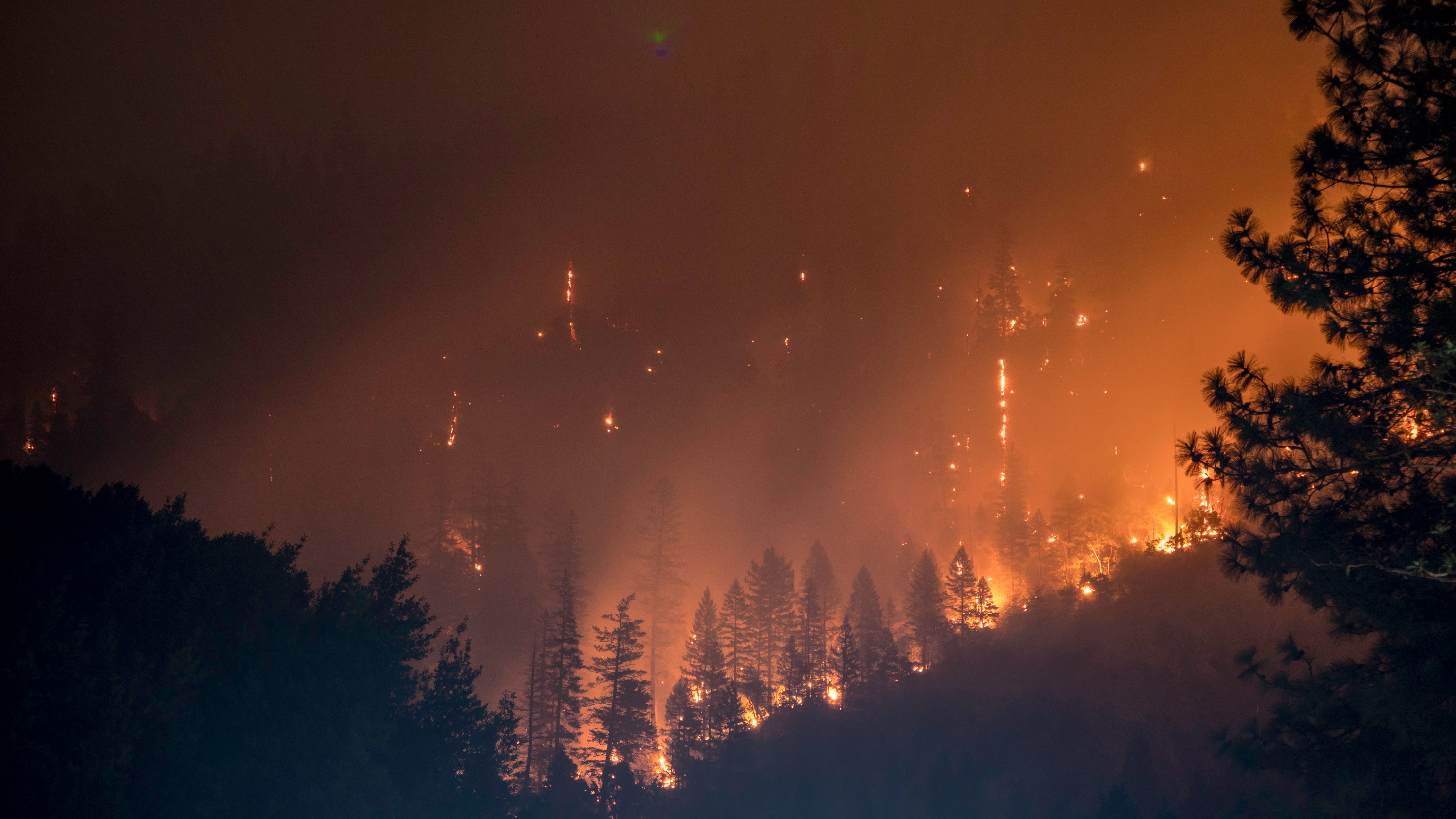
Photo by Matt Howard on Unsplash
Forest fires are one of the major natural catastrophes.
They can endanger both human and wild life. And can severely destruct the environment.
This is why predicting forest fires accurately is important.
In this project, I used data to explore forest fires that occurred in the Montesinho Natural Park in Portugal. My goal was to see how data can be used to predict the amount of danger caused by the fires.
I used R language for the data analysis. The codebase is shared on GitHub.
This dataset was collected by the researchers Cortez and Morais during the time from January 2000 to December 2003. You can find the complete dataset on the UCI Machine Learning Repository.
Where is Montesinho Natural Park?
Now, you may be interested to know about the park the data is coming from. It's one of the largest natural parks in Portugal, with an area of 74,230 hectares.
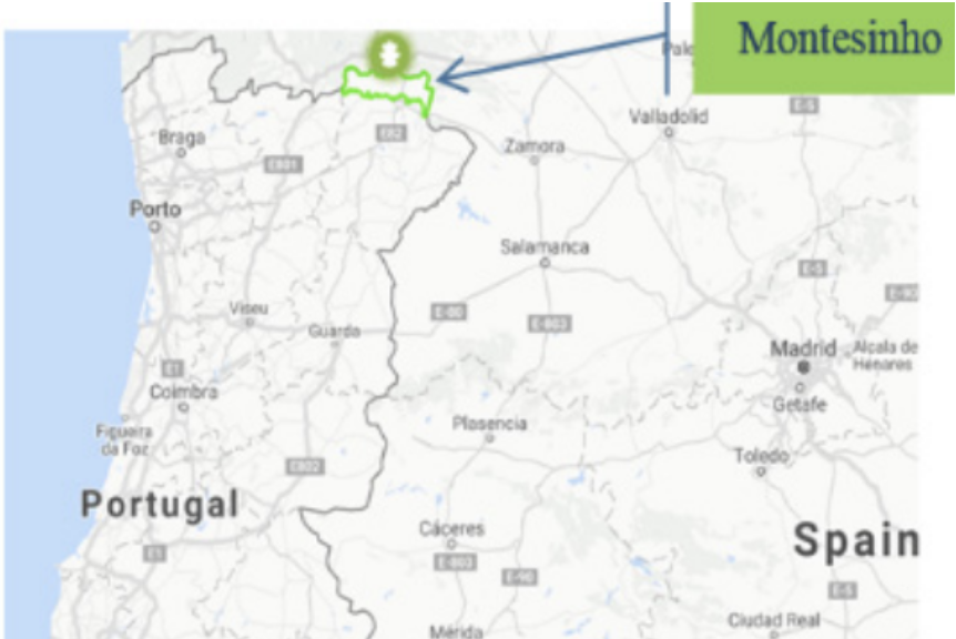
Location of Montesinho Natural Park
Montesinho has a diverse natural habitat with 240 species of animals. Annual temperature of the park varies from 8 to 120C, although the temperature in summer could reach up to 400C.

Montesinho Natural Park (Image by Elisha.wolf, CC BY-SA 4.0, via Wikimedia Commons)
About the Dataset
Each row in the dataset is about a fire that had occurred in the park. There are 517 entries, described using 13 variables.
The image below summarises the 13 variables in the dataset. They are categorised into categorical variables, fire weather indexes and weather conditions. The amount of area burnt by fire is used as the target variable.
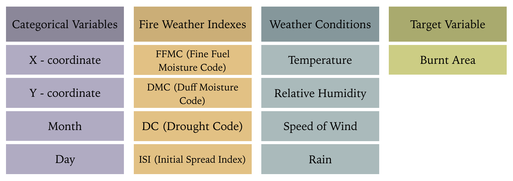
Figure 1: Variables in the dataset
The fire weather indexes FFMC, DMC, DC and ISI in the above variables are defined in the Fire Weather Index (FWI). They indicate the danger of the fire based on weather conditions. The higher these indexes are, the more dangerous the fire could be.
FFMC indicates the fuel moisture content in forest litter, while DMC indicates the fuel moisture of decomposed organic material. DC determines long-term moisture conditions, and ISI measures the speed of fire spread.
Problem to solve
The purpose of this project is predicting the burnt area of a fire in Montesinho Park based on variables such as location, weather conditions and fire indexes.
Data Transformations
Before working on any data analysis, the target variable 'burnt area' needed to be transformed. After plotting the target variable, we can see that more than 47% of the values are zero (first histogram below). To reduce this skewed distribution, I took the logarithmic value (second histogram). As the target variable should be positive (since area should be a positive value), the log(area+1) transformation was used (third histogram).
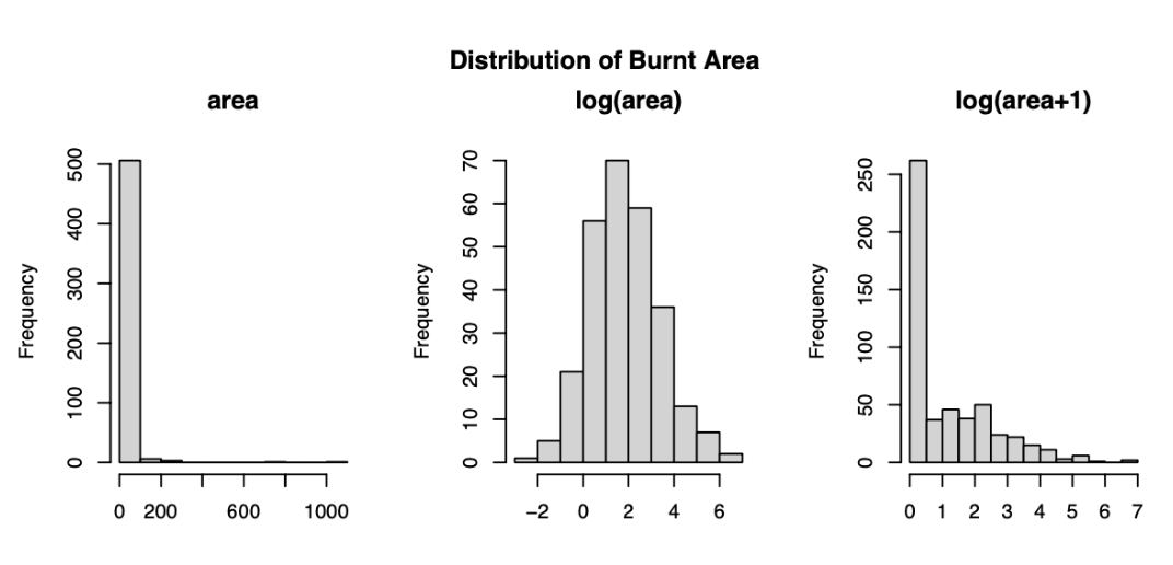
Figure 2: Distribution of target variable before and after transformation
Exploring Data
Linear correlation
To start off with, I looked at the linear relationship and correlation among the variables in the dataset. The scatter plots below show the distribution of target variable against the 12 independent variables. The plots don't show any clear indication of linear relationship among the variables. When examining the Pearson correlation for numerical variables, the variable 'DMC' had the highest positive correlation of 0.067 with target variable 'Burnt area', which shows very small linear relationship.
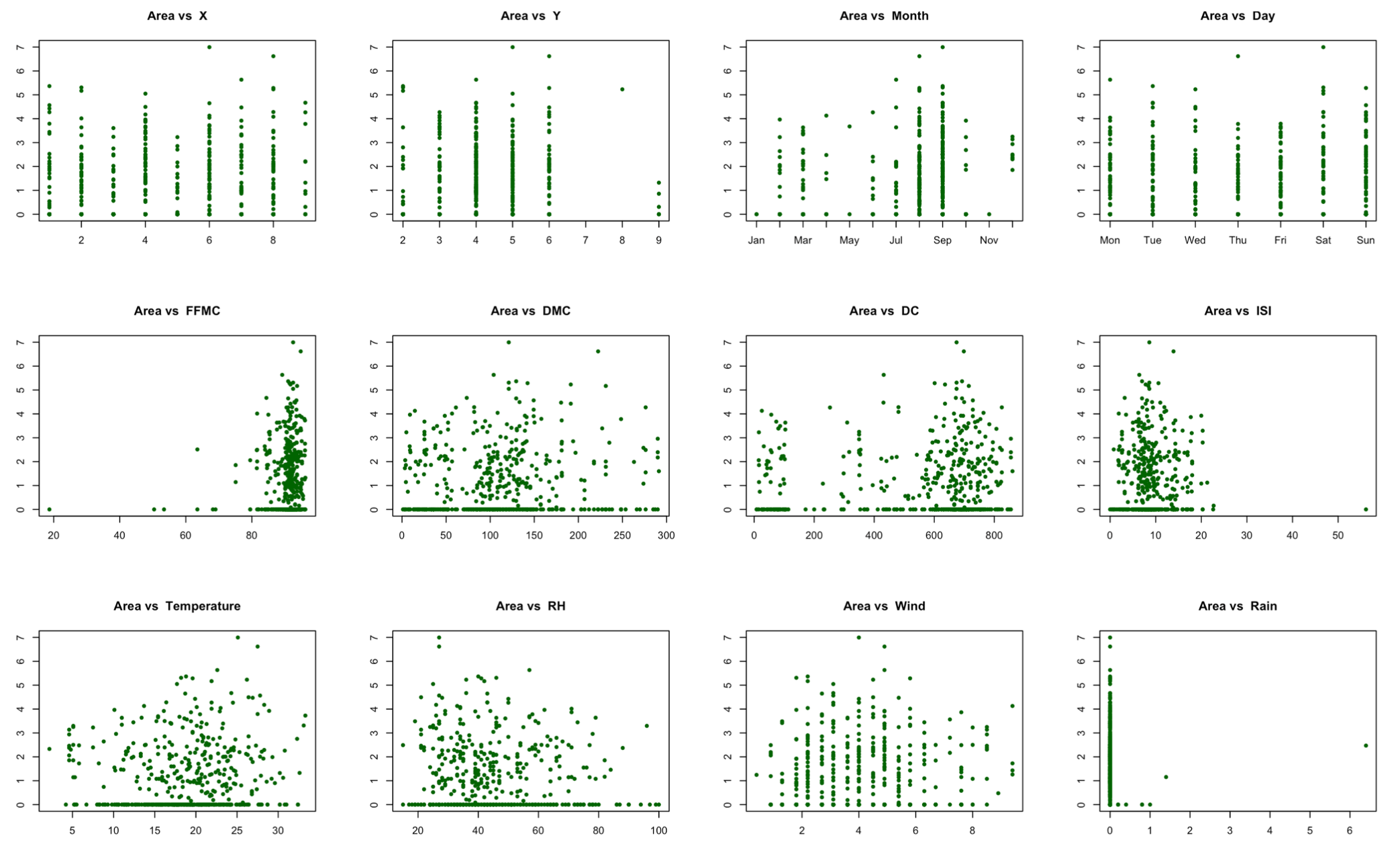
Figure 3: Scatter plots of target variable against dependent variables
Because there is little evidence about any linear correlation among variables, next I looked at the dataset-specific aspects. The 4 categorical variables—x and y coordinates and Month and Day capture geographical and temporal information in the dataset.
Fire intensity by location
Therefore, first I used the x and y coordinates to generate a heatmap and identify the areas that were more prone to fires. The generated heatmap below show the areas outside the park in green, while the park is in heatmap colours. As we can see in the map, most of the heavy fires had been contained in the edges of the park, while the middle of the park had faced less severe fires. However, as the leftmost edge of the park has areas with less severe fires close to highly burnt areas, we can decide that fires have not spread rapidly across the park.
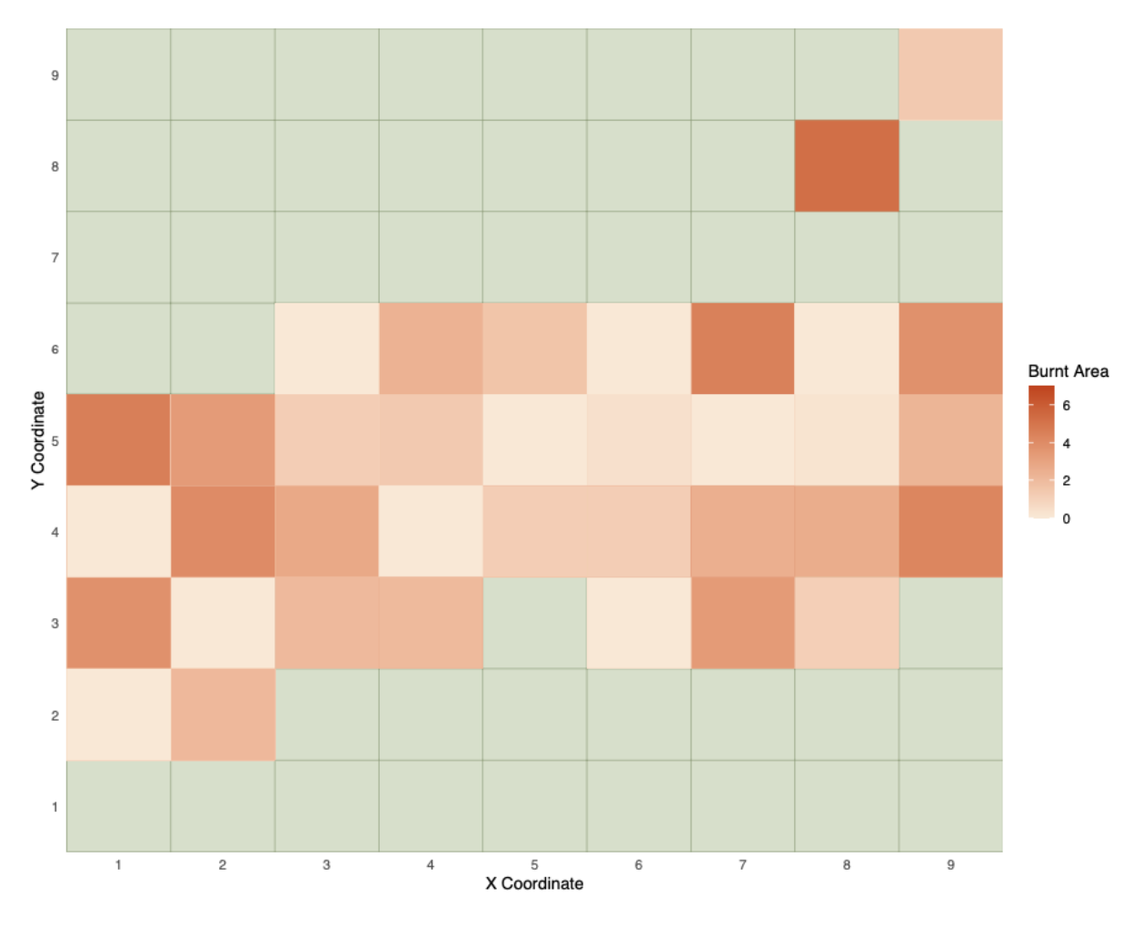
Figure 4: Heatmap of burnt areas in the park using location coordinates
Fire intensity by season
Next, I used the month attribute to find if fires had any seasonal variations. The scatter plot below shows occurrence of fires across the four seasons. As expected, we can see that there had been more fires during summer and autumn compared to the low frequency of fires in winter and spring. However, it's difficult to identify a clear pattern among burnt area and the season, as we can see many fires with an area of zero during summer, while some fires in winter have had burnt areas with the values 2 and 4.
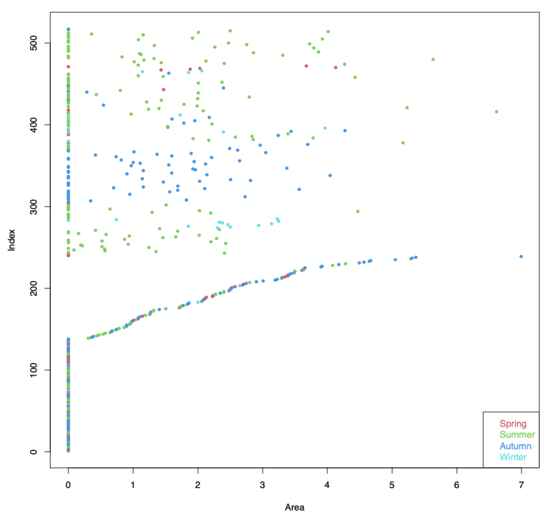
Figure 5: Variation of burnt area by seasons
Data Analysis using non-linear regression
Since the dataset didn't show any evident linear correlation, I used non-linear regression with the numerical variables.
To further explore the nature of relationship among variables, I used the pair plot below.
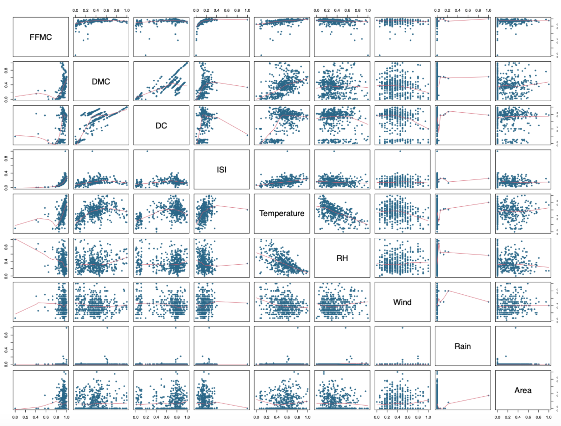
Figure 6: Pair plots for numerical variables
The last row of the above pair plot shows the variation of Area against each predictor variable. We can see that Temperature has an evident curve in its graph, indicating a possible non-linear relationship. Similarly, if we disregarded the outlier points in the graphs of FFMC and ISI, we can see that majority of data points have a curved distribution. Considering these behaviours, I added the variables as polynomial terms to the model with an order of 2.
So far we have,
Area = ... + Temperature^2 + ISI^2 + FFMC^2 + ...
Then, I considered the relationships among variables to add the interaction terms to the model. If two predictors did not show any evident relationship among each other, they were added as interaction terms to the model.
For instance, Temperature and Wind variables show an equally spread set of points, which does not show a clear connection. Therefore, the combination of Temperature and Wind was added to the model as an interaction term. Another example is the plot of Wind against ISI, which shows that ISI has a curved relationship with Wind. Therefore, an interaction term with a polynomial term was added to the model as ISI2 * Wind.
After training the model, variables that had a low significance (high P-value) such as ISI and RH were removed
to improve the model.
The model became,
Area =  FFMC + DMC + DC + Temperature + Wind + Rain + Temperature^2 + ISI^2 + FFMC^2 + DMC^2 + Wind^2 + DC*ISI +
        FFMC*ISI + RH*Wind*Rain + Temperature*Wind + Temperature*DMC + ISI2*Wind
nolin_model1 <- lm(Area ~ .+ I(Temperature^2) + I(ISI^2) + I(FFMC^2) + I(DMC^2) + I(Wind^2) + DC*ISI + RH*Wind*Rain
+ Temperature*Wind + I(ISI^2)*Wind + FFMC*ISI
+ Temperature*DMC -ISI -RH, data = fire_norm)
summary(nolin_model1)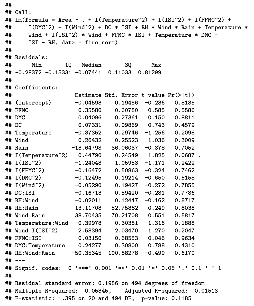
Figure 7: Summary of initial non-linear model
This model had a high R2 value of 0.05345, but the adjusted R2 of the model was 0.01513. The significant gap between these values show that the model is not well generalised and may over fit the data. We can see this in the low significance of majority of variables in the model.
Improving the model
Removing variables with high P-values (low significance) helped to improve the significance of the model. The resulting model was as follows:
Area = FFMC + DC + Temperature + Temperature2 + FFMC2 + Wind2 + DC*ISI + RH*Rain + ISI2*Wind# simplified model
nolin_model2 <- lm(Area ~ .+ I(Temperature^2) + I(FFMC^2)
+ I(Wind^2) + DC*ISI + RH*Rain + I(ISI^2)*Wind
-ISI -RH -DMC -Rain -Wind, data = fire_norm)
summary(nolin_model2)
Figure 8: Summary of improved non-linear model
This model gave an R2 value of 0.04602 which was lower than the R2 from the initial non-linear model of 0.05345. However, the improved model had more significant terms, of which Temperature2 had the highest significance with three stars and a P-value of 0.000907. Temperature and DC had high significances with two- and one-star ratings respectively. The interaction term RH*Rain had a significance rating of one dot (.), with a P-value of 0.063176. The adjusted R2 was 0.02709, which gave a reduced difference between the R2 values.
To sum up, the implemented model shows that weather conditions such as temperature, rain, relative humidity and Drought Code (DC) play an important role in defining the severity of fires.
To find more interesting effects of each parameter, we can cluster data to find similar data points and build separate regression models for each group.